First MC/DC Simulation
This guide presupposes you are familiar with modeling nuclear systems using a Monte Carlo method. If you are completely new, we suggest checking out OpenMC’s theory guide as most the basic underlying algorithms and core concepts are the same. Our input decks and keyword phrases are designed so that if you are familiar with tools like OpenMC or MCNP, you should be able to get up and running quickly.
While this guide is a great place to start, the next best place to look when getting started are our MCDC/examples or MCDC/test directories.
Run a few problems there, change a few inputs around, and keep looking around until you get the general hang of what we are doing.
Believe it or not, there is a method to all this madness.
If you find yourself with errors you really don’t know what to do with, take look at our GitHub issues page.
If it looks like you are the first to have a given problem feel free to submit a new ticket!
A note on testing: Just because something seems right doesn’t mean it is. Care must be taken to ensure that you are running the problem you think you are. The software only knows what you tell it.
MC/DC Workflow
MC/DC uses an input -> run -> post-process workflow, where users
build input decks using scripts that import
mcdcas a package and call functions to build geometries, tally meshes, and set other simulation parameters,define a runtime sequence in the terminal to execute the
inputscript (terminal operations are required for MPI calls),export the results from
.h5files and use the MC/DC visualizer or tools likematplotlibto view results.
Building an Input Script
Building an input deck can be a complicated and nuanced process. Depending on the type of simulation you need to build, you could end up touching most of the functions in MC/DC, or very few.
Again, the best way to start building input decks is to look at what we have already done in the MCDC/examples or MCDC/test directories.
To see more on the available input functions, look through the Input Definition section.
As an example, we walk through building the input for the MCDC/test/regression/slab_absorbium problem, which simulates a three-region, purely absorbing, mono-energetic slab wall.
We start with our imports:
import numpy as np

import mcdc
You may require more packages depending on the methods you are constructing, but most of what you need will be in these two. Now, we define the materials for the problem:
# Set materials
m1 = mcdc.MaterialMG(capture=np.array([1.0]))
m2 = mcdc.MaterialMG(capture=np.array([1.5]))
m3 = mcdc.MaterialMG(capture=np.array([2.0]))
In this problem we only have mono-energetic capture, but MC/DC has support for multi-group (capture, scatter, fission) and continuous energy (capture, scatter, fission).
Multi-group materials are created with mcdc.MaterialMG; for example, a 3-group capture cross section would be capture=np.array([1.0, 1.1, 0.8]).
Continuous-energy materials are created with mcdc.Material.
If you are a member of CEMeNT, we have internal repositories containing the data required for continuous-energy simulation. Unfortunately due to export controls we can not publicly distribute this data. If you are looking for cross-section data to plug into MC/DC, we recommend you look at OpenMC or NJOY.
After setting material data, we define the problem space by setting up surfaces with their boundary conditions.
If no boundary condition is defined, the surface is assumed to be internal (boundary_condition="none").
Surfaces are created using class methods on mcdc.Surface (e.g., PlaneX, PlaneY, PlaneZ, Sphere, CylinderZ).
# Set surfaces
s1 = mcdc.Surface.PlaneZ(z=0.0, boundary_condition="vacuum")
s2 = mcdc.Surface.PlaneZ(z=2.0)
s3 = mcdc.Surface.PlaneZ(z=4.0)
s4 = mcdc.Surface.PlaneZ(z=6.0, boundary_condition="vacuum")
Remember that the radiation transport equation is a 7-dimensional integro-differential equation, so it’s possible your problem will need both initial and boundary conditions. While we have tried to include warnings and errors if an ill-posed problem is detected, we cannot forecast all the ways in which things might go haywire. For transient simulations, initial conditions are assumed to be 0 everywhere.
We create problem geometry using cells, which are defined by the surfaces that constrain them and the material that fills them.
The +/- convention is used to indicate whether the cell volume is outside (+) or inside (-) a given surface.
For example, below, the first cell is filled with material m2 and is positive with respect to s1, negative with respect to s2.
This corresponds to being bound on the left by s1 and on the right by s2.
Cells are created with mcdc.Cell, using the region and fill keyword arguments.
mcdc.Cell(region=+s1 & -s2, fill=m2)
mcdc.Cell(region=+s2 & -s3, fill=m3)
mcdc.Cell(region=+s3 & -s4, fill=m1)
We define a uniform isotropic source throughout the domain:
mcdc.Source(z=[0.0, 6.0], isotropic=True, energy_group=0)
Next we set tallies and specify the specific parameters of interest. Here, we’re interested in the space-averaged flux
and collision rate. A mesh is created first, then a mesh-filtered Tally is constructed on that mesh.
Direction bins can also be specified on the tally.
Regardless of problem specifics, particles are simulated through all space, direction, and time;
the tally definitions are used to indicate in which dimensions a record of particle behavior should be kept.
Available tracklength scores include "flux", "density", "collision", "capture", and "fission".
Current tallies can be attached to either a surface or a cell.
Current scoring uses the surface-crossing estimator in both cases.
For explicit surface filters, supported score is "current-net".
For cell filters, supported scores are "current-net", "current-in", and "current-out".
The "current-in" and "current-out" scores are positive partial currents; "current-net" keeps the sign
of the crossing direction.
# Tally: cell-average fluxes and collisions
mesh = mcdc.MeshStructured(z=np.linspace(0.0, 6.0, 61))
mcdc.Tally(
    mesh=mesh,
    scores=["flux", "collision"],
    mu=np.linspace(-1.0, 1.0, 32 + 1),
)

# Tally: current crossing a cell boundary
mcdc.Tally(
    cell=my_cell,
    scores=["current-net", "current-in", "current-out"],
)
Next we set simulation settings. The only required setting is the number of particles.
Settings are configured by assigning attributes on the mcdc.settings singleton.
Additional settings include, for example, the cycles to use for a k-eigenvalue problem
(via mcdc.settings.set_eigenmode(...)) or the output file name.
mcdc.settings.N_particle = 1000
Finally, execute the problem.
mcdc.run()
Put together, our example input.py file:
import numpy as np
import mcdc

# =============================================================================
# Set model
# =============================================================================
# Three slab layers with different purely-absorbing materials

# Set materials
m1 = mcdc.MaterialMG(capture=np.array([1.0]))
m2 = mcdc.MaterialMG(capture=np.array([1.5]))
m3 = mcdc.MaterialMG(capture=np.array([2.0]))

# Set surfaces
s1 = mcdc.Surface.PlaneZ(z=0.0, boundary_condition="vacuum")
s2 = mcdc.Surface.PlaneZ(z=2.0)
s3 = mcdc.Surface.PlaneZ(z=4.0)
s4 = mcdc.Surface.PlaneZ(z=6.0, boundary_condition="vacuum")

# Set cells
mcdc.Cell(region=+s1 & -s2, fill=m2)
mcdc.Cell(region=+s2 & -s3, fill=m3)
mcdc.Cell(region=+s3 & -s4, fill=m1)

# =============================================================================
# Set source
# =============================================================================
# Uniform isotropic source throughout the domain

mcdc.Source(z=[0.0, 6.0], isotropic=True, energy_group=0)

# =============================================================================
# Set tally, setting, and run mcdc
# =============================================================================

# Tally: cell-average fluxes and collisions
mesh = mcdc.MeshStructured(z=np.linspace(0.0, 6.0, 61))
mcdc.Tally(
    mesh=mesh,
    scores=["flux", "collision"],
    mu=np.linspace(-1.0, 1.0, 32 + 1),
)

# Setting
mcdc.settings.N_particle = 1000

# Run
mcdc.run()
Now that we have a script to run, how do we actually run it?
Running a Simulation
MC/DC supports execution purely in the Python interpreter, compiled to CPUs (x86, ARM64 and Power9-64), and GPUs (AMD and Nvidia) and supports threading with MPI (Python or compiled modes). Other guides are included to execute in these modes but for the sake of this first MC/DC simulation we will simply execute in Python mode (slower, no acceleration) simply with
python input.py
from a command line. For more performance see how to execute MC/DC on CPUs and GPUs
Postprocessing Results
While the entire workflow of running and post-processing MC/DC could be done in one script, unless the problem is very small (or you’re an expert), we recommend using separate simulation and post-processing/visualization scripts.
When a problem is executed tallied results are compiled, compressed, and saved in .h5 files.
The size of these files can vary widely depending on your tally settings,
the geometric size of the problem (e.g. number of surfaces), and the number of particles tracked.
Expect sizes as small as kB or as large as TB.
These result files can be exported, manipulated, and visualized.
Data can be pulled from an .h5 file using something like,
import h5py
import numpy as np
# Load results
with h5py.File("output.h5", "r") as f:
    # The tally name matches the auto-generated name (e.g., "mesh_tally_0")
    tally_name = list(f["tallies"].keys())[0]
    tally = f[f"tallies/{tally_name}"]

    z = tally["grid/z"][:]
    dz = z[1:] - z[:-1]
    z_mid = 0.5 * (z[:-1] + z[1:])

    mu = tally["grid/mu"][:]
    dmu = mu[1:] - mu[:-1]
    mu_mid = 0.5 * (mu[:-1] + mu[1:])

    psi = tally["flux/mean"][:]
    psi_sd = tally["flux/sdev"][:]
While there can be some nuance to the dimensions of these data arrays, the folder structures should be evident from your tally settings.
You can see the structure of the file layer-by-layer using the keys attribute of an h5 group.
For example, f.keys() will return
<KeysViewHDF5 ['runtime', 'tallies']>
and f['tallies'].keys() will list all tally names.
If needed, you can look around a .h5 file using something like h5Viewer (which on linux can be installed with sudo apt-get install hdfview).
Otherwise these arrays can then be manipulated and modified like any other.
Results are stored as NumPy arrays, so any tool that works with NumPy arrays (e.g., SciPy and Pandas)
can be used to analyze the data from your simulations.
A tool like matplotlib will work great for plotting results.
For more complex simulations, open source professional visualization software like
Paraview or Visit are available.
As the problem we ran above is pretty simple and has no scattering or fission, we have an analytic solution we can import:
from reference import reference
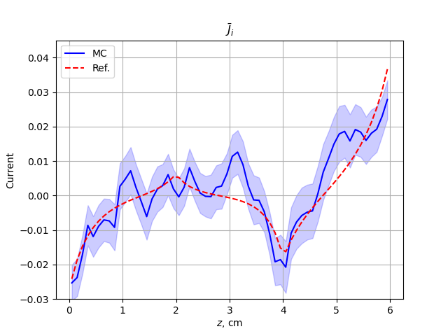
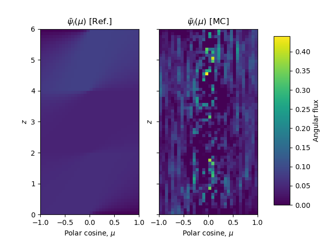
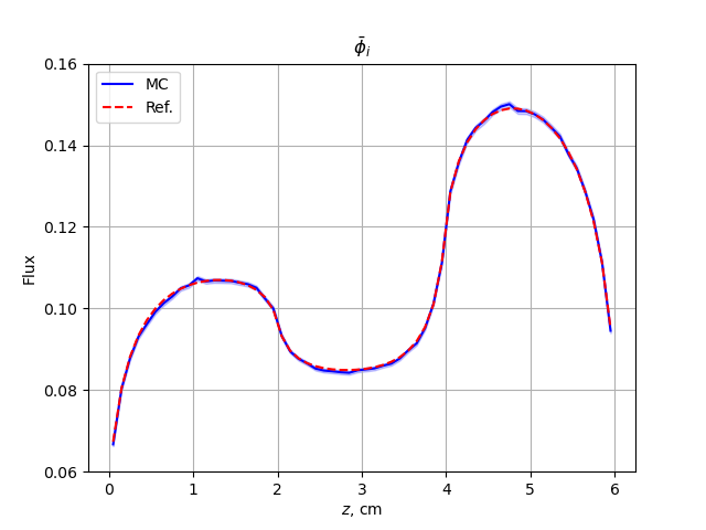
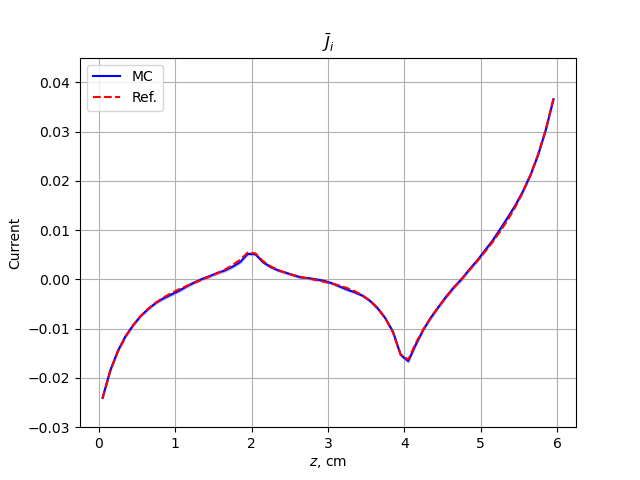
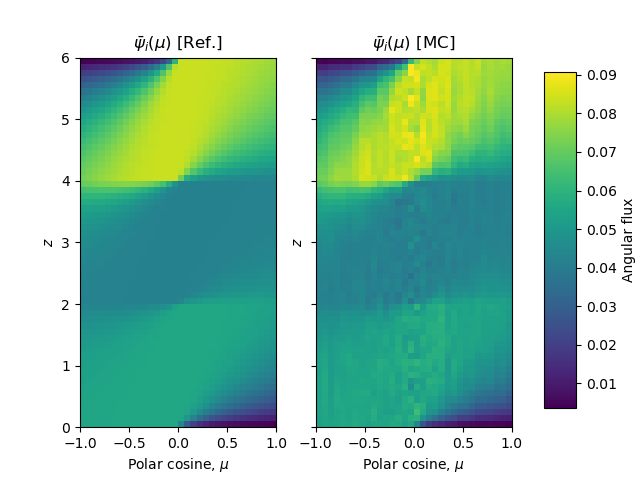
In the script below, we plot the space-averaged flux and space-averaged current, including their statistical noise. We also use the space-averaged flux and current to compute a new quantity, the space-averaged angular flux, and plot it over space and angle in a heat map. Remember that when reporting results from a Monte Carlo solver, you should always include the statistical error!
import matplotlib.pyplot as plt
import numpy as np

I = len(z) - 1
N = len(mu) - 1

# Scalar flux
phi = np.zeros(I)
phi_sd = np.zeros(I)
for i in range(I):
    phi[i] += np.sum(psi[i, :])
    phi_sd[i] += np.linalg.norm(psi_sd[i, :])

# Normalize
phi /= dz
phi_sd /= dz
J /= dz
J_sd /= dz
for n in range(N):
    psi[:, n] = psi[:, n] / dz / dmu[n]
    psi_sd[:, n] = psi_sd[:, n] / dz / dmu[n]

# Reference solution
phi_ref, J_ref, psi_ref = reference(z, mu)

# Flux - spatial average
plt.plot(z_mid, phi, "-b", label="MC")
plt.fill_between(z_mid, phi - phi_sd, phi + phi_sd, alpha=0.2, color="b")
plt.plot(z_mid, phi_ref, "--r", label="Ref.")
plt.xlabel(r"$z$, cm")
plt.ylabel("Flux")
plt.ylim([0.06, 0.16])
plt.grid()
plt.legend()
plt.title(r"$\bar{\phi}_i$")
plt.show()

# Current - spatial average
plt.plot(z_mid, J, "-b", label="MC")
plt.fill_between(z_mid, J - J_sd, J + J_sd, alpha=0.2, color="b")
plt.plot(z_mid, J_ref, "--r", label="Ref.")
plt.xlabel(r"$z$, cm")
plt.ylabel("Current")
plt.ylim([-0.03, 0.045])
plt.grid()
plt.legend()
plt.title(r"$\bar{J}_i$")
plt.show()

# Angular flux - spatial average
vmin = min(np.min(psi_ref), np.min(psi))
vmax = max(np.max(psi_ref), np.max(psi))
fig, ax = plt.subplots(1, 2, sharey=True)
Z, MU = np.meshgrid(z_mid, mu_mid)
im = ax[0].pcolormesh(MU.T, Z.T, psi_ref, vmin=vmin, vmax=vmax)
ax[0].set_xlabel(r"Polar cosine, $\mu$")
ax[0].set_ylabel(r"$z$")
ax[0].set_title(r"\psi")
ax[0].set_title(r"$\bar{\psi}_i(\mu)$ [Ref.]")
ax[1].pcolormesh(MU.T, Z.T, psi, vmin=vmin, vmax=vmax)
ax[1].set_xlabel(r"Polar cosine, $\mu$")
ax[1].set_ylabel(r"$z$")
ax[1].set_title(r"$\bar{\psi}_i(\mu)$ [MC]")
fig.subplots_adjust(right=0.8)
cbar_ax = fig.add_axes([0.85, 0.15, 0.05, 0.7])
cbar = fig.colorbar(im, cax=cbar_ax)
cbar.set_label("Angular flux")
plt.show()
While this script does look rather long, most of these commands are controlling things like axis labels and whatnot. But at the end we have something like this.
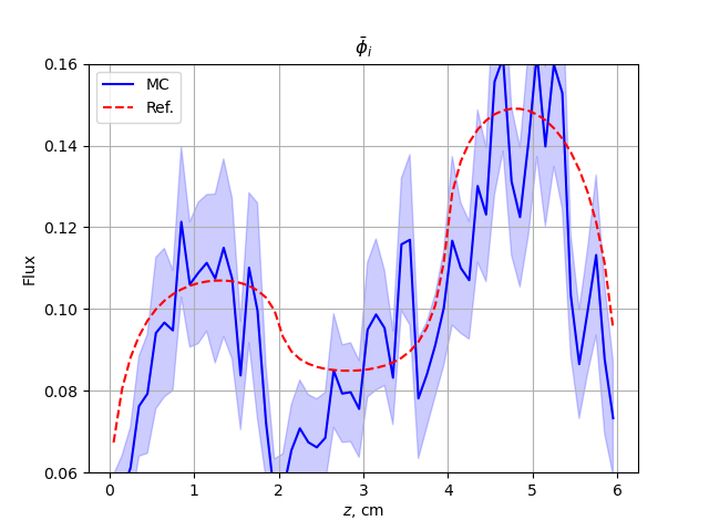
Notice how noisy these solutions are? We only ran 1e3 particles. We need more particles to get a less statistically noisy, more converged solution. Here’s results from the same simulation run with 1e6 particles:
This is much better converged around the analytic solution. As with everything else, the best way to see what you can do is sniff around the examples. We have examples with animated solutions, subplots, moving regions and more!
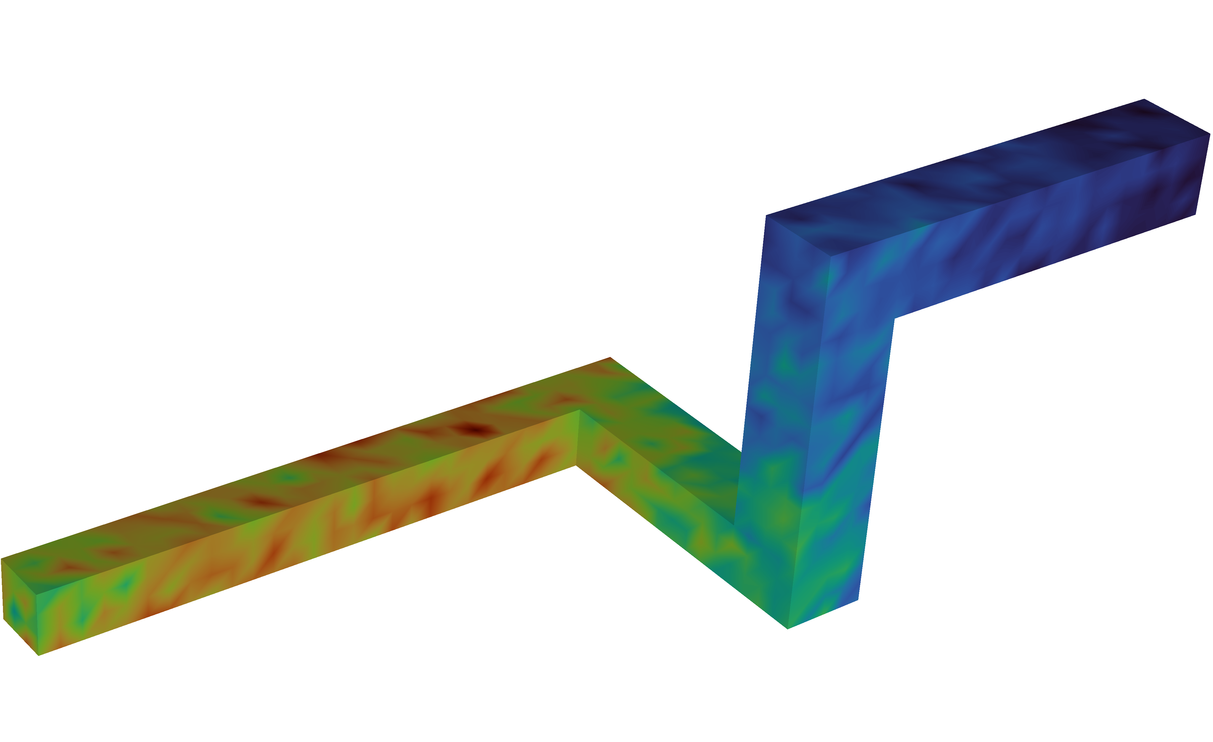
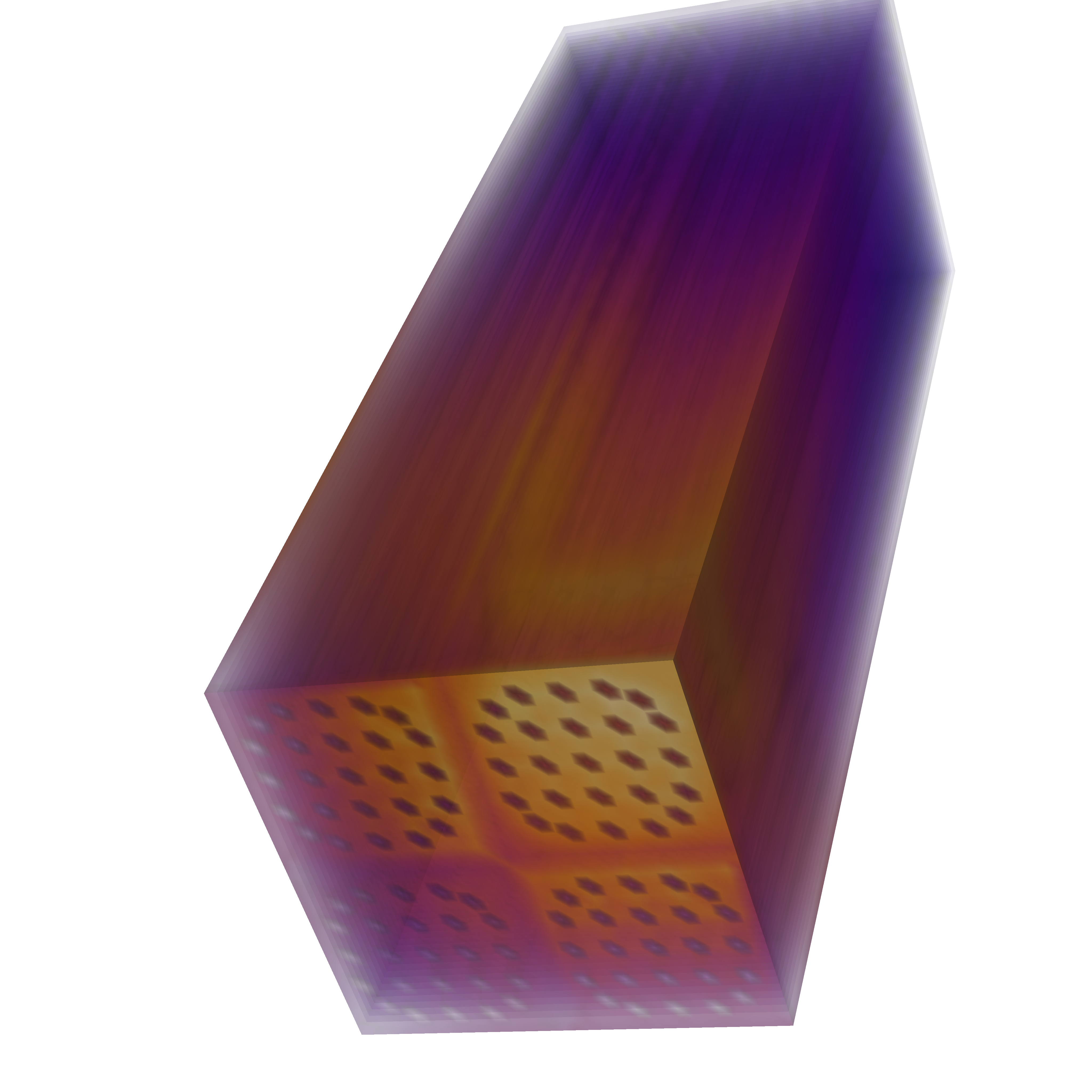
Additional Simulation Results
Neutron flux distribution on a shielded dog-leg vacuum channel after a neutron pulse is completed
Bottom-view of a micro reactor fission rate distribution when a control rod-driven runaway prompt supercritical occurs
Fission and flux bursts of a neutron excursion driven by a drop of highly-enriched uranium.