
Runtime Data Layout#
After model compilation has discovered, finalized, and ordered the Python object graph, mcdc.main.prepare calls generate_numba_layers in mcdc.code_factory to create the runtime representation used by transport.
The representation has two complementary parts:
simulationA fixed-layout NumPy structured record containing scalar state, embedded records, typed object collections, fixed-size arrays, and metadata.
dataA contiguous one-dimensional NumPy array containing variable-length numerical payloads and lists of object IDs.
The same logical representation is supplied to Python, Numba-CPU, and Numba-GPU execution. Portable transport code expresses its state through this prepared representation. See Python-First, Numba-Accelerated Design for this development model.
Why Two Structures?#
Python model objects may contain arrays whose sizes depend on the problem: energy grids, cross sections, mesh boundaries, motion tables, tally filters, and many others. Nested Python object references and variable-sized arrays cannot be embedded directly in the stable NumPy structured dtype required by the Numba execution modes. Separating fixed-layout metadata from variable-length values keeps the structured dtype stable while accommodating model-dependent payloads.
Runtime Object Model#
Fixed fields become structured-record fields, Python object references become simulation-local IDs, and variable-length fields become offsets into data.
Generated mcdc_get and mcdc_set accessors perform the corresponding lookups and offset calculations.
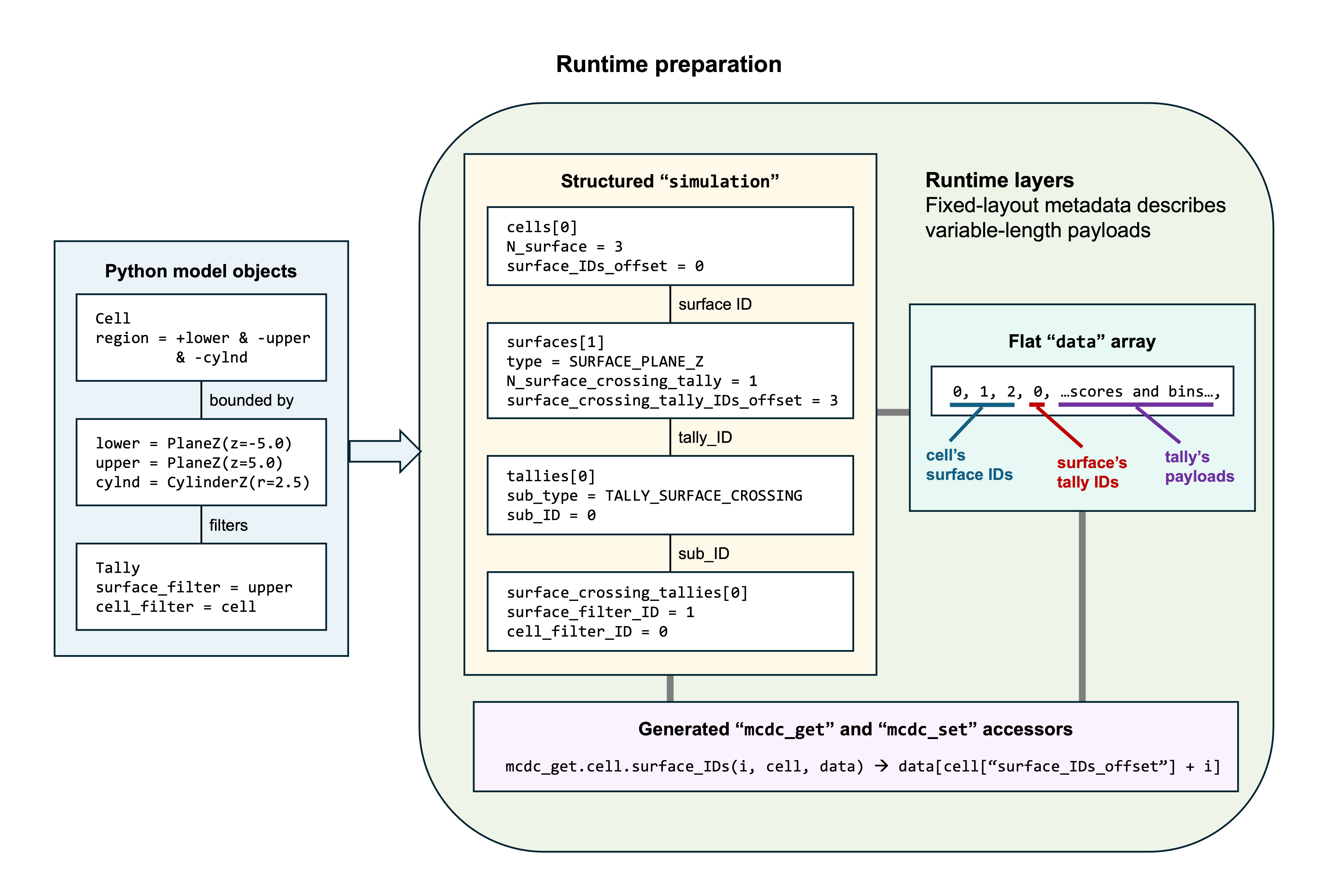
The figure follows one connected example from Python model objects into the two runtime layers.
The cell record locates its three surface IDs in data, the selected surface record locates an attached tally ID, and the base tally record identifies its concrete surface-crossing record.
Tally scores, bins, and other variable-length payloads share the same flat arena.
The IDs and offsets shown in the figure are illustrative; their values depend on the compiled model and its packed layout.
The data arena uses float64 values, one allocation, and one offset space across execution modes.
Integer values stored in the arena, including object IDs, are restored to their declared types by generated scalar accessors.
Object Collections#
Registered model objects are stored in collections on simulation.
The figure demonstrates both forms of runtime collection: direct indexing for non-polymorphic objects and base-to-concrete dispatch for polymorphic objects.
For a non-polymorphic category, an object’s simulation-local ID directly indexes its collection. A particle’s current cell and one of its boundary surfaces are therefore retrieved with:
cell = simulation["cells"][particle["cell_ID"]]
surface_ID = mcdc_get.cell.surface_IDs(0, cell, data)
surface = simulation["surfaces"][surface_ID]
A polymorphic category has both a common base collection and a collection for each concrete representation.
A surface stores the IDs of the surface-crossing tallies attached to it.
Each ID first selects a base tally record, whose sub_type and sub_ID identify the concrete surface-crossing record:
from mcdc.constant import TALLY_SURFACE_CROSSING


tally_ID = mcdc_get.surface.surface_crossing_tally_IDs(0, surface, data)
tally = simulation["tallies"][tally_ID]

tally["sub_type"] == TALLY_SURFACE_CROSSING  # True

surface_crossing_tally = simulation["surface_crossing_tallies"][tally["sub_ID"]]
The concrete tally record retains surface_filter_ID and cell_filter_ID, connecting it back to the selected surface and cell.
All IDs are assigned during model compilation and identify objects only within the current simulation snapshot.
The hierarchy and ID assignment are described in Simulation Compilation.
Variable-Length Fields#
Using the illustrative values in the figure, the cell and selected surface records store metadata equivalent to:
cell.surface_IDs_offset = 0
cell.N_surface = 3

surface.surface_crossing_tally_IDs_offset = 3
surface.N_surface_crossing_tally = 1
The corresponding ID lists occupy adjacent regions of data in the simplified layout:
data[0:3] = [0, 1, 2]  # Cell's surface IDs
data[3:4] = [0]        # Surface's tally ID
Array Shapes and Generated Access#
Array shape annotations determine whether an array is embedded in a structured record or stored in data.
For example, Cell.translation has a completely fixed shape:
translation: Annotated[NDArray[float64], (3,)]
Because every dimension is an integer literal, the three-component array is embedded directly in the cell record and accessed through cell["translation"].
Surface.move_velocities combines a model-dependent dimension with a fixed trailing dimension:
move_velocities: Annotated[NDArray[float64], ("N_move", 3)]
The symbolic dimension N_move names the surface record field that supplies its size at runtime.
Because that dimension depends on the model, the array is flattened into data, and the surface record stores its offset and total length.
Fully symbolic multidimensional arrays use the same mechanism.
For example, NeutronMultigroupData.nu_d is shaped ("G", "J") and uses the
named energy-group and delayed-neutron-group dimensions to reconstruct indexing
into its flattened payload.
Generated accessors for arrays stored in data currently support array ranks from one through four dimensions.
mcdc.code_factory generates modules under mcdc/mcdc_get and mcdc/mcdc_set for fields stored in data.
These helpers hide offset and stride arithmetic from transport code and remain callable from both Python and Numba-compiled functions.
Conceptually, a generated element getter for the cell’s surface IDs performs:
from numpy import int64


def surface_IDs(index, cell, data):
    offset = cell["surface_IDs_offset"]
    return int64(data[offset + index])
Transport code can therefore express logical access without depending on where the values reside in data:
surface_ID = mcdc_get.cell.surface_IDs(index, cell, data)
For move_velocities, the generated accessor uses the fixed trailing dimension as the row stride and reconstructs logical two-dimensional indexing:
velocity = mcdc_get.surface.move_velocities(
    move_index, component_index, surface, data
)
For NeutronMultigroupData.nu_d, the generated element getter reads the named
trailing dimension J from the neutron-model record and uses it as the
runtime row stride:
def nu_d(group, delayed_group, neutron_multigroup, data):
    offset = neutron_multigroup["nu_d_offset"]
    stride = neutron_multigroup["J"]
    return data[offset + group * stride + delayed_group]
In the row-major flattened layout, J determines the stride between energy groups, while G determines the number of rows.
Generated helpers also provide operations for complete arrays, final elements, chunks, vectors, and multidimensional elements as appropriate.
Scalar getters restore the integer type declared by an annotation or implied by an object-ID list.
Bulk getters continue to return zero-copy float64 views into data and therefore require explicit conversion when an integer array is needed outside transport.
Deriving the Layout#
Classes in mcdc/object_ declare their runtime-visible fields with Python type annotations.
generate_numba_layers collects those annotations and maps them to runtime fields:
Scalars become scalar structured fields.
Fixed-shape annotated arrays are embedded in structured records.
Variable-length arrays become
<field>_offsetand<field>_lengthmetadata plus values indata.Object references become
<field>_IDfields.Lists of object references become
N_<object>and<object>_IDs_offsetmetadata plus IDs indata.Members named in a class’s
non_numbalist are excluded from the packed representation or handled specially.
Packing is performed in two passes:
Walk the compiled objects to build records and calculate the required
datasize.Allocate
dataand walk the objects again to copy flattened payloads into their assigned regions.
The structured simulation dtype can then be finalized because collection sizes, particle-bank sizes, and nested record types are known.
Generated Numba Support and Problem-Dependent Dtypes#
The derived layout feeds artifacts with three different lifetimes:
- Generated Numba support
mcdc/numba_types.pyand the modules undermcdc/mcdc_getandmcdc/mcdc_setdescribe the runtime schema developed in the preceding sections. These generated source files are shared by every simulation using that MC/DC source tree. They change with the object model or Numba support generator, not with an input problem.- Problem-dependent dtypes
Each call to
mcdc.main.preparederives collection lengths, particle-bank capacities, and other sizes from one compiled model. Pure factories inmcdc.numba_typesuse those sizes to return simulation and particle-bank dtypes local to that preparation. The factories do not install the returned dtypes in shared module globals.- Prepared runtime state
generate_numba_layersuses the problem-dependent dtypes to allocate and pack that simulation’ssimulationanddataobjects. This state is owned by the prepared simulation and used during transport.
This separation allows independent processes to run differently sized problems from the same installation. Each process creates and retains its own problem-dependent dtypes, while the generated Numba support remains read-only.
Import and Preparation Order#
Generated Numba support is established at the process level:
Importing
mcdcloads the complete object model.mcdc.configparses-ror--rebuildwith the other command-line options, and package initialization calls its MPI-aware rebuild gate. When rebuilding is requested, rank zero regenerates the Numba support and the other ranks in that MPI launch wait for it to finish.Runtime modules may then import
numba_types,mcdc_get, andmcdc_set.
This process-level step does not depend on a mcdc.Simulation or its
compilation. Each simulation is subsequently compiled and prepared using the
support already established during import. Preparation creates fresh
problem-dependent dtypes and prepared runtime state for that simulation.
The MPI barrier coordinates ranks within one launch, not independent launches. Independent jobs sharing an MC/DC source tree must use previously generated, read-only Numba support. See Rebuilding Numba Support for the object model development workflow and rebuild commands.
Static Constants and Simulation-Specific Literals#
MC/DC distinguishes static implementation constants from values derived for one prepared simulation.
mcdc.constant defines stable codes, event flags, numerical limits, and tolerances that have the same meaning for every simulation.
These values can be imported directly by the model, transport, and output layers.
Some compiled operations instead require a simulation-dependent value to be known as a Numba literal.
During mcdc.main.prepare, make_literals in mcdc.code_factory.literals_generator derives those values from the compiled Python model and replaces the placeholder functions in mcdc.literals with JIT-compatible implementations that return them.
The current example is the work-array size used to evaluate cell-region reverse Polish notation. The generator finds the largest required evaluation buffer in the compiled model, and geometry transport obtains that value through:
value = util.local_array(
    literals.rpn_evaluation_buffer_size(),
    np.bool_,
)
Use a generated literal only for a single simulation-wide value that compiled code must treat as fixed during the prepared run.
Store values that vary by object or particle in the structured simulation state or data instead.
Because literals are derived from a particular model snapshot, runtime preparation regenerates them whenever that simulation is prepared again.
The One-element Container#
The generated simulation record is stored in a one-element NumPy array:
simulation_container, data = prepare(simulation_python)
simulation = simulation_container[0]
The container gives Python, Numba, MPI, and GPU paths a consistent mutable reference to the structured state.
Transport drivers receive the container and data; individual kernels generally operate on the record or its nested objects.
Transport Consumption#
Portable transport functions shared across the execution backends consume the runtime representation and primitive transport records. They use:
Direct structured-field access for fixed-size values and metadata.
Base and subtype IDs to navigate registered objects.
mcdc_getandmcdc_setfor variable-length values.The same function signatures in Python and Numba-CPU modes.
The layout is fixed for the duration of a prepared run. Transport may update allocated values, tally bins, particle banks, and runtime counters, but it cannot resize a field or introduce a new model object. Changing the prepared MC/DC model requires a new model compilation and runtime preparation pass.
Execution Backends#
Continue with Transport Execution to see how Python, Numba-CPU, and Numba-GPU consume this shared layout.